
If you missed the first blog on this subject, then have a quick read to get the overview of what I am describing this this series. Advanced XL Contract Manager – Overview
RAG Status
RAG literally stands for Red, Amber, Green and forms the basis for an easy win for building a dashboard and reporting. When implementing a RAG model, it is very important to make a clear statement of what each level equates to, for instance:
- Green – process/contract on target and on time, no major issues/risks
- Amber – process/contract over budget or delayed. Some issues, but manageable
- Red – serious issue/risk process likely to fail without senior management support
By setting clearly defined parameters for each level, selecting the right one will be easier and when an amber or red flag is seen, the level of concern and attention is quickly allocated.
Process Stage
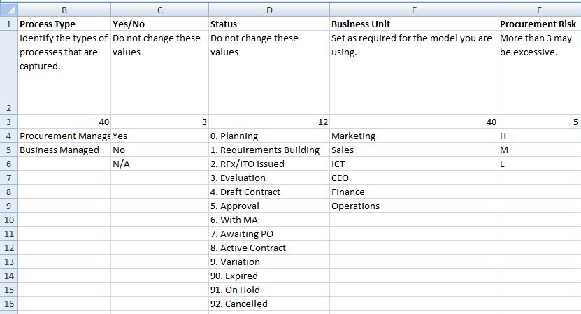
Since we are going to use this application for more than just tracking our completed contracts, we need a method of flagging what stage the process is up to. Due to the sorting quirks of Excel, putting a numeric value as a prefix will provide some advantages. Consider the key stages your organisation uses, but as a guide you could use:
1: Planning
2: Requirements Building
3: Offer Released
4: Evaluation
5: Draft Contract
6:Approval
7: Active Contract
8: Expired
9.1: On Hold
9.2: Cancelled
Action
An active contract will have to come to an end at some stage, or maybe a variation will occur during the life of the contract. This is where the Action functionality kicks in, so the next step/current requirement can be tracked. Examples of actions are:
- Variation
- Terminate
- Expire
- Renew
- Replace
Project or Programme
This field allows the grouping of contracts with no relationship other than they are for the same project. You may have a contract for a resource, another for software and a third for establishing accommodation in a new building for the project team. By including this field, these disparate contracts can be quickly recalled and reviewed.
Endorsed Process
If the organisation has a challenge to overcome maverick spending, then capturing the incidence of contracts that were established without using the approved methodology will provide a powerful reporting opportunity. This could be s simple yes/no field, or the reason for not being endorsed can be capture , such as “insufficient quotes”, “poor documentation”, “no procurement support”, “order splitting”, etc.
Procurement Methodology/Strategy
This will provide tremendous capacity to review the common practices of procurement within the organisation. How often are single processes used, are open tenders common, what percentage of the contracts are bought from sole providers. The model we’ll build in this solution will provide a two tier structure of the strategy selected and the method used to deliver the strategy.
Full list of fields
For a full list of the fields used, download the sheet from the PME4U Procurement Resources page.
Data Validation
If you gain nothing else from this article, even if you do not go on to implement the full solution, what I am about to explain here will make a huge difference to the quality of data captured in any spreadsheet you develop.
When we look at any data capture spreadsheet, we will see fields that should only have a limited number of options entered. If the data entered isn’t consistent, then our ability to search, group, sort or filter will be limited or completely disabled. Consider the Process Stage and Action fields I mentioned above, what are the chances of them being consistently entered if they were just free text fields? Not good.
 Think about a simple yes/no field. You think that there are only two options, but over time you will see variations such as “yes”, “y”, “no”, “n”. Then you will get the occasional “x”. In fact, without validation, completely random information will accidentally find its way into the field. Data validation in its simplest form will fix this issue.
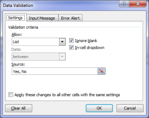
For a basic yes/no field. Simply select the field, click on the Data ribbon and select the Data Validation option. In the Allow field choose List and then in the Source field type “yes, no” (without the quotes) and save. When you click back in the field you will notice that there is now a drop down that offers only the options you just typed. If you type “y” and hit enter you will get an error message.
One problem solved and for many, this is a eureka moment. But this solution is very limited. Imagine you have 10 fields in your document that use the yes/no validation and you decide you now want to add an “N/A” option. You have to make the validation change in 10 fields. What if you have a list of options that you want end users to maintain such as names of departments or products, but you don’t want them playing around with the validation settings?
The more flexible and dynamic solution is the validation rule that uses a dynamic named range.
Where a spreadsheet is going to have one or more validated value lists, it is good idea to include a worksheet to hold those lists. I generally call it something obvious like “Lookups”. Now, to capture the values you store in columns of the Lookups sheet, you will need to use Named Ranges.
The basic named range simply gives a name to a single cell or a range of cells, which makes recalling that range more intuitive and can make formulas easier to read (but more about that in a later post). On the Lookups sheet, in cell A1 type “Yes” then in A2 type “No”. Select both cells and then in the Name Box in the top left (above the “A” column and it probably has “A2” or “A3” displayed now) type in “YesNo” and hit enter.
You have just created a named range called “YesNo”. Lets put that to use now. In your contracts list, pick a field that requires a yes no answer. With that cell selected, go to the Data ribbon and select Data Validation. Select List in Allowed but this time in the Source field hit the F3 key on your keyboard. This will display a list of all the Names in the workbook. Pick our new “YesNo” Name and click ok.
Going back to our cell in the contracts list, we find the drop down arrow with our two allowed values. Nifty huh. But what if we want to add “N/A” as an option?
On the Lookups sheet, add “N/A” at the bottom of the list. Nip back over to the contracts list and check our validation field and…uh ho…it isn’t there.
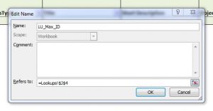
This is a weakness in the basic use of the Named range. But here is the next cool thing, a named range isn’t a named range, it is in fact a named formula. Go to the Formulas tab on the ribbon and open the Name Manager. Note the format of the field called “Refers to”. In this case it is “=Lookups!$J$4”.
 So the beauty of a Named Formula, as it should be called, is that we can put almost any formula Excel formula or function in here. We can use them to define a constant such as a Name called “Tax” with a Refers to of “=0.12”. We can then create a formula in a cell in a worksheet that states “= G3*Tax” and the result in that field would be the value of G3 multiplied by 0.12.
Knowing this opens up a lot of opportunities for optimising our worksheets, and for our immediate need, optimise our validation look ups. Here we are going to use the Offset function within our named formula. It has a syntax of OFFSET( range, rows, columns, [height], [width] ).
This function allows us to set a start point (range), then shift that start point down (rows) and right (columns) from that start point, and then define an area (height and width) that we are interested in. Take a look at the the screenshot of the Lookups sheet. Don’t worry about the values in rows 2 and 3, we’ll cover their purpose in a later blog. How can we capture the values in the Business Unit list and make it so anyone can update the list and immediately add the value to all our validation fields that use it? Looking at the Offset function, we would add in the formula of “=OFFSET(E1,3,0,13,1)”. This starts us from cell E1, shifts us down 3 rows to E4, doesn’t move us right at all, then sets an area 13 rows high by 1 wide. In effect, have achieved the same as the previous example, but in a much more complicated way, but if we replace the value of thirteen with a COUNTA function, it gets a whole lot cleverer. The new formula would be (E1,3,0,COUNTA(Lookups!E:E)-3,1). Now the height of the area is dependent on the number of contiguous values listed. Add another value at the bottom of the list, and like magic, the area extends and the new value will appear in all validations using this Named Formula. For a little more detail, the COUNTA function is used rather than the COUNT function as it handles text and numeric values in the list and the “-3” simply removed the count of the first three rows because we start counting from the top of the column. I could have set the “range” value as E4, but if that value were ever deleted, it would result in a #REF error in the named formula, so it is better to start from a field that will never be deleted.
So now our Named Formula/Range should look like this:
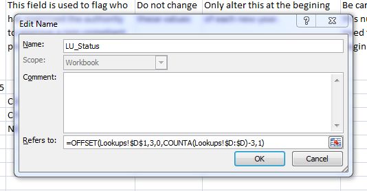
Using the Named Formula in our validation is exactly the same as the previous process, so set that up. Check you get a list of the current values, then add some new values to the bottom of the list and like magic, they will appear in your drop down validation list.
You can use the same functionality to have a horizontal named range that dynamically spans columns by changing the count function look along a row and then shift it into the last argument space like this (D1,3,0,1,COUNTA(Lookups!2:2)).
Note also the naming convention I have used, the prefix of “LU_” lets me know this is a range on the Lookups sheet. This becomes very important when you add dozens of named formulas in a complex workbook and in some cases you may define a Name for a range that holds the “Number” on the maintenance, register, dashboard. Using the prefix you can call them all “Number”.
Here is a quick video demonstrating the whole process:
http://www.youtube.com/watch?v=t2Jpwx7ls6Q
As a side note, when learning new tricks in Excel, the internet is your best friend. If you have a problem, use your favourite search engine to track down an answer. I have to say a big thanks to Ozgrid.com for this brilliant trick.
So play around with this new bit of knowledge, download the example workbook and start building those skills. In the next blog, we’ll jump into the concept of separating the raw data from the viewing and maintenance functions by building a Lookups Maintenance function.